
Transformer: Attention is All You Need
1. Overall Architecture
The Transformer is a sequence-to-sequence neural architecture based entirely on self-attention mechanisms, without recurrence or convolution. It consists of two main parts:
- Encoder: Generates contextualized representations of input sequences.
- Decoder: Autoregressively generates output sequences based on encoder output and previously generated tokens.
Figure: Transformer Architecture
Step 1: Input Embedding
Input takes word embedding and position embedding, and adds them together. The result is passed to the encoder.
\[\text{Input} = \text{Embedding}(x) + \text{PositionEmbedding}(x)\]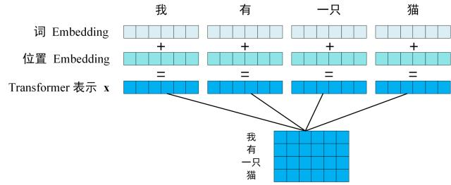
Figure: Transformer Input Embedding
Step 2: Encoder
Input vector is represented as a matrix $X \in \mathbb{R}^{n \times d_{\text{model}}}$, where $n$ is the sequence length and $d_{\text{model}}$ is the embedding dimension. The encoder consists of $N$ identical layers, each with two sub-layers:
- Multi-head self-attention (MHA)
- Feed-forward network (FFN)
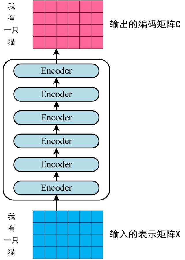
Figure: Encoder Process
Step 3: Decoder
The decoder also consists of $N$ identical layers, each with three sub-layers:
- Masked multi-head self-attention (MHA)
- Multi-head self-attention (MHA) with encoder output as keys and values
- Feed-forward network (FFN)
The use of Masked MHA ensures that the prediction for a given position depends only on the known outputs at previous positions.
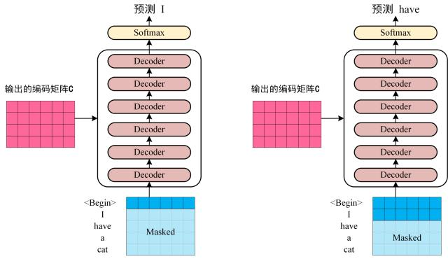
Figure: Decoder Prediction
Step 4: Output
The decoder output is passed through a linear layer followed by a softmax function to produce the final output probabilities for the next token in the sequence.
\[\text{Output} = \text{softmax}(\text{DecoderOutput} \times W_{\text{embedding}}^T)\]Where $W_{\text{embedding}}$ is the learned embedding matrix. The softmax function converts the logits into probabilities for each token in the vocabulary.
2. Input of Transformer
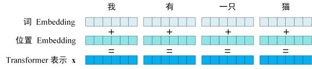
Figure: Transformer Input
2.1 Word Embedding
- Input tokens are mapped to embedding vectors using learned embeddings.
- Embedding dimension: $d_{\text{model}}$ (typically 512).
2.2 Positional Embedding
- Added to embeddings to inject positional information.
- Fixed sinusoidal positional embeddings used:
3. Self-Attention
3.1 Architecture of Self-Attention
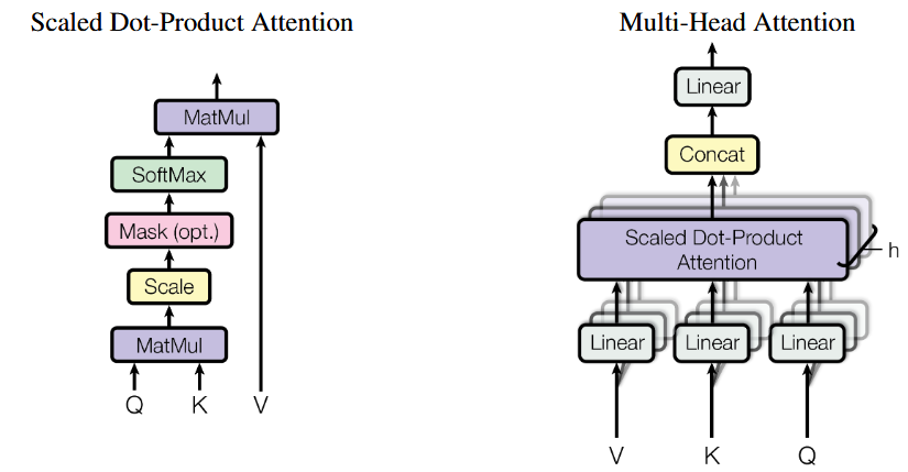
In practice, we compute the attention function on a set of queries simultaneously, packed together into a matrix $Q$. The keys and values are also packed together into matrices $K$ and $V$.
Self-attention maps queries (Q), keys (K), and values (V) to an output via scaled dot-product attention:
\[\text{Attention}(Q, K, V) = \text{softmax}\left(\frac{QK^T}{\sqrt{d_k}}\right)V\]- $Q, K, V$: matrices of queries, keys, and values.
- $d_k$: dimension of queries and keys.
3.2 Calculating Q, K, V
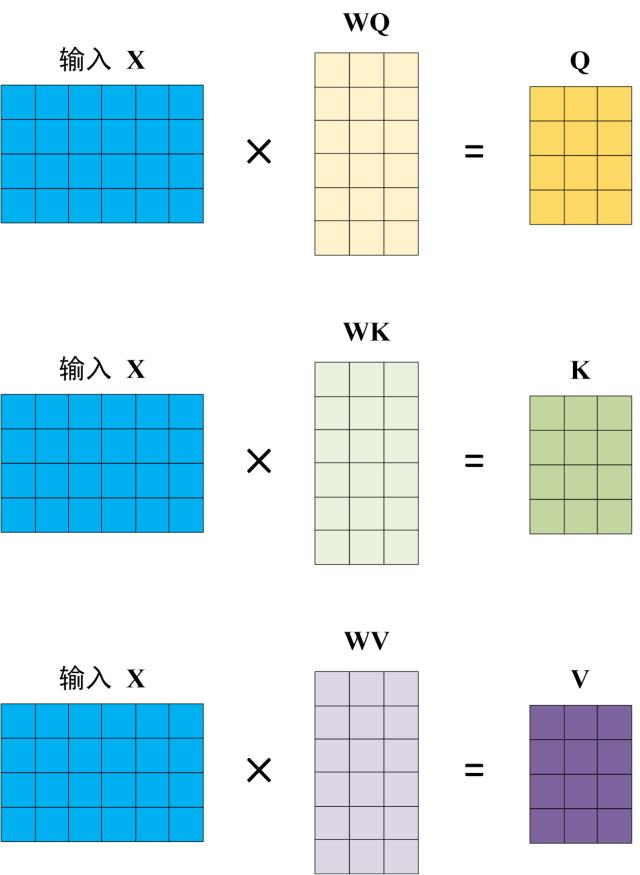
Figure: Calculating Q, K, V
Computed via learned linear projections from input embeddings ($X$):
\[Q = X W^Q,\quad K = X W^K,\quad V = X W^V\]Where $W^Q, W^K, W^V$ are learned parameter matrices.
First calculate the $Q K^T$:
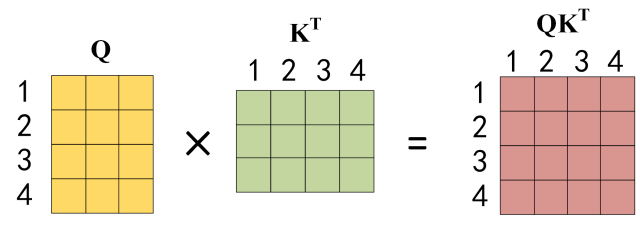
Figure: Calculating $Q K^T$
Then apply the softmax function to each row to get the attention weights:
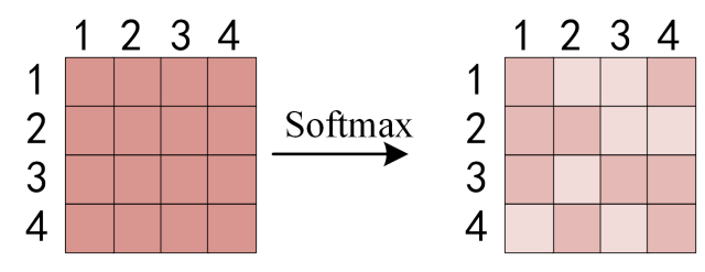
Figure: Apply softmax on rows
Multiply the attention weights with the values to get the output:
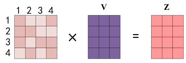
Figure: Multiply values
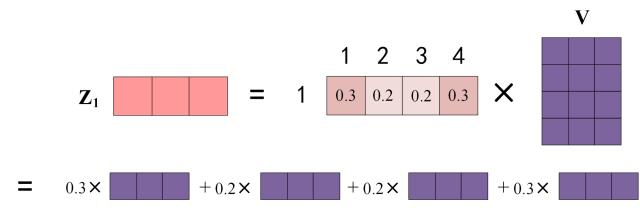
Figure: Get Output Z
3.3 Output of Self-Attention
- Weighted sum of values based on attention scores.
- Output dimension matches input embedding size ($d_{\text{model}}$).
3.4 Multi-Head Attention (MHA)
Multiple parallel attention heads run independently, then concatenate:
\[\text{MultiHead}(Q, K, V) = \text{Concat}(\text{head}_1, \dots, \text{head}_h) W^O\]Each head computes:
\[\text{head}_i = \text{Attention}(Q W_i^Q, K W_i^K, V W_i^V)\]- Typically, $h=8$, each head dimension $d_k = d_v = d_{\text{model}}/h$.
4. Architecture of Encoder

4.1 Add and LayerNorm
Each encoder layer includes residual connections and layer normalization:
\[x = \text{LayerNorm}(x + \text{Sublayer}(x))\]- Applied after Multi-head Self-Attention and Feed-Forward layers.
4.2 Feed Forward
Position-wise fully-connected feed-forward network (FFN):
\[\text{FFN}(x) = \max(0, xW_1 + b_1)W_2 + b_2\]- Intermediate dimension typically $d_{ff}=2048$.
4.3 Input and Output Calculation of Encoder
Overall encoder-layer calculation per layer:
\[x = \text{LayerNorm}(x + \text{MultiHeadSelfAttn}(x))\] \[x = \text{LayerNorm}(x + \text{FFN}(x))\]- Encoder stack repeats this structure $N=6$ times.
5. Architecture of Decoder
Decoder consists of 6 identical layers, each with three sub-layers.
5.1 First MHA in Decoder Block
- Masked self-attention prevents tokens from attending to future positions.
- Computation is similar to encoder self-attention, but with a causal mask:
5.2 Second MHA in Decoder Block (Encoder-Decoder Attention)
- Queries come from previous decoder sub-layer.
- Keys and values come from the final encoder output:
5.3 Softmax Prediction
- After decoder stack, the final decoder representation is projected to vocabulary logits:
- Softmax function predicts next token probabilities:
References
Transformer Architecture provides a powerful parallelizable structure for sequence modeling, relying entirely on attention mechanisms to encode global dependencies efficiently.