From Q-learning to Soft Actor Critic

We shall introduce the foundation of value-base RL algos, Q-learning. Then from Q-learning to DQN, A2C, and finally to SAC.

1. Background: Q-Learning

1.1 What is a Q?

In reinforcement learning, an agent interacts with a Markov Decision Process (MDP), defined by:

• A set of states $\mathcal{S}$
• A set of actions $\mathcal{A}$
• Transition dynamics $P(s’ \mid s, a)$
• A reward function $r(s, a)$
• A discount factor $\gamma \in [0, 1]$

State value function $V^\pi(s)$

The state-value function under a policy $\pi$ is defined as the expected return when starting in state $s$ and following $\pi$ thereafter:

\[V^\pi(s) = \mathbb{E}_{\pi} \left[ \sum_{t=0}^{\infty} \gamma^t r(s_t, a_t) \mid s_0 = s \right]\]

Action value function $Q^\pi(s, a)$

The action-value function under policy $\pi$ is the expected return starting from state $s$, taking action $a$, and then following policy $\pi$:

\[Q^\pi(s, a) = \mathbb{E}_{\pi} \left[ \sum_{t=0}^{\infty} \gamma^t r(s_t, a_t) \mid s_0 = s, a_0 = a \right]\]

So compared to state value function, there is an action in this function.

Relationship Between $Q^\pi(s, a)$ and $V^\pi(s)$

The value of a state can be expressed as the expected value over actions drawn from the policy:

\[V^\pi(s) = \mathbb{E}_{a \sim \pi(\cdot|s)} \left[ Q^\pi(s, a) \right]\]

Thus, $Q$ quantifies how good an action is at a given state, while $V$ quantifies how good the state is, under a specific policy.

1.2 What is Q-Learning?

Q-learning is a model-free, off-policy algorithm that learns the optimal action-value function $Q^*(s, a)$, defined as:

\[Q^*(s, a) = \max_{\pi} Q^\pi(s, a)\]

That is, $Q^{*}(s, a)$ gives the expected return of taking action $a$ in state $s$ and thereafter following the optimal policy $\pi^{*}$.

1.2.1 Bellman Optimality Equation for $Q^*$

Q-learning is based on the Bellman optimality equation:

\[Q^*(s, a) = \mathbb{E}_{s'} \left[ r(s, a) + \gamma \max_{a'} Q^*(s', a') \right]\]

This equation is recursive and serves as a fixed-point definition for the optimal Q-function.

Bootstrapping and Backup

Q-learning updates are bootstrapped — meaning they rely on the agent’s own current estimates to update future values. Unlike Monte Carlo methods, which wait for full returns at the end of an episode, Q-learning performs online updates using a one-step target:

\[\text{TD target} = r + \gamma \max_{a'} Q(s', a')\]

Here, $Q(s’, a’)$ is not the true value but the agent’s current estimate. This is the essence of bootstrapping — updating based on estimated values rather than ground truth.

Additionally, Q-learning implements a backup operation — information from the successor state $s’$ is backed up to improve the current estimate $Q(s, a)$:

\[Q(s, a) \leftarrow Q(s, a) + \alpha \left[ \underbrace{r + \gamma \max_{a'} Q(s', a')}_{\text{backed-up estimate}} - Q(s, a) \right]\]

This is a one-step backup, where the immediate reward and the estimated value of the next state are used to update the current value.

These concepts are central to temporal difference (TD) learning and are what make Q-learning both sample-efficient and incremental.

1.2.2 Q-learning Update Rule

At each step, the agent observes a transition $(s, a, r, s’)$ and updates the Q-value:

\[Q(s, a) \leftarrow Q(s, a) + \alpha \left[ r + \gamma \max_{a'} Q(s', a') - Q(s, a) \right]\]

Where:

• $\alpha$ is the learning rate
• $\gamma$ is the discount factor
• The term in brackets is the temporal difference (TD) error

This is a form of stochastic approximation toward the fixed point of the Bellman optimality equation.

1.2.3 Policy Iteration in Q-Learning

Q-learning can be interpreted as performing a form of generalized policy iteration (GPI), alternating between:

Policy Evaluation (Approximate)

Unlike classical policy evaluation (which assumes a fixed policy), Q-learning bootstraps the evaluation by updating $Q(s,a)$ based on one-step lookahead:

• Uses the greedy action in the next state to evaluate the current state-action pair.
• Does not wait for convergence — hence approximate.

Policy Improvement (Implicit)

At any point, we can extract a greedy policy from $Q$:

\[\pi(s) = \arg\max_a Q(s, a)\]

This defines the greedy policy, which becomes optimal as $Q(s,a)$ converges to $Q^*(s,a)$.

Although Q-learning does not explicitly represent a policy, it implicitly improves the policy by making $Q(s,a)$ closer to the optimal, and selecting better actions during planning or execution.

1.3 Theoretical Justification

Q-learning is a stochastic approximation algorithm that converges to the fixed point of the Bellman optimality operator:

Let the Bellman operator be:

\[\mathcal{T}Q(s, a) = \mathbb{E}_{s'} \left[ r(s, a) + \gamma \max_{a'} Q(s', a') \right]\]

This operator is a $\gamma$-contraction in the sup-norm:

\[\| \mathcal{T}Q_1 - \mathcal{T}Q_2 \|_\infty \leq \gamma \| Q_1 - Q_2 \|_\infty\]

Therefore, by Banach’s Fixed Point Theorem, repeated application of $\mathcal{T}$ converges to a unique fixed point: the optimal Q-function $Q^*$.

1.4 Training Q-Learning

At a high level, the Q-learning training loop consists of:

1. Initialize $Q(s,a)$ for all $s \in \mathcal{S}$, $a \in \mathcal{A}$
2. Repeat (for each episode or step):
   • Observe current state $s$
   • Choose action $a$ (e.g., using $\epsilon$-greedy policy)
   • Execute $a$ in the environment
   • Observe reward $r$ and next state $s’$
   • Update $Q(s, a)$ using the Bellman target
   • Update $s \leftarrow s’$
3. Continue until convergence

Choose an action

At state $s$, select action $a$ using an exploration policy:

• Commonly, $\epsilon$-greedy:

\[\begin{cases} \text{with probability } \epsilon & \text{choose a random } a \in \mathcal{A} \\ \text{with probability } 1 - \epsilon & a = \arg\max_{a'} Q(s, a') \end{cases}\]

Update Q-Value

Apply the Q-learning update rule:

\[Q(s, a) \leftarrow Q(s, a) + \alpha \left[ r + \gamma \max_{a'} Q(s', a') - Q(s, a) \right]\]

This moves the estimate $Q(s, a)$ toward a better approximation of $Q^*(s, a)$ using the one-step target:

\[\text{TD target} = r + \gamma \max_{a'} Q(s', a')\]

And it’s also called TD target.

The TD error is:

\[\delta = \text{TD target} - Q(s, a)\]

1.5 Summary of Q-Learning

Q-learning is a foundational off-policy reinforcement learning algorithm that estimates the action-value function:

\[Q(s, a) \leftarrow Q(s, a) + \alpha \left[ r + \gamma \max_{a'} Q(s', a') - Q(s, a) \right]\]

• Learns the value of taking an action in a state.
• The policy is implicitly derived from the Q-function:
  \(\pi(s) = \arg\max_a Q(s, a)\)
• Works well for discrete action spaces with small state/action counts.

Q-learning converges under certain conditions:

• The learning rate $\alpha_t(s, a)$ decays appropriately: $\sum_t \alpha_t(s,a) = \infty$ $\sum_t \alpha_t^2(s,a) < \infty$
• Each state-action pair is visited infinitely often.
• The environment is a stationary MDP.

2. Deep Q-Networks (DQN)

DQN extends Q-learning using deep neural networks to approximate the Q-function in high-dimensional or continuous state spaces.

2.1 Motivation: Why Move Beyond Q-Learning

While Q-learning provides a theoretically grounded framework for value-based reinforcement learning, its practical application in high-dimensional or continuous environments is limited due to challenges in approximation, stability, and sample efficiency.

Limitations of Classical Q-Learning with Function Approximators:

1. Instability with Nonlinear Function Approximators: When combined with function approximators such as neural networks, Q-learning’s bootstrapped updates can lead to divergence or oscillations. This is due to:
   • Correlations in sequential data
   • Non-stationary targets
   • Feedback loops between the Q-function and the target
2. Sample Inefficiency: Standard Q-learning updates use each transition exactly once and immediately discard it. This is inefficient, especially in environments where data collection is expensive.
3. Poor Generalization Across Similar States: Without proper architecture and training regularization, function approximators may overfit to individual transitions rather than generalizing well over the state space.
4. Lack of Stabilization Mechanisms: Classical Q-learning assumes exact updates and idealized convergence properties. In practice, approximators require architectural tools (e.g., target networks) to stabilize training.

These practical challenges necessitated the development of Deep Q-Networks (DQN) — a realization of Q-learning that integrates neural function approximation with a set of stabilization techniques.

2.2 Deep Q-Network (DQN): Core Idea

DQN replaces the Q-table with a neural network parameterized by $\theta$, approximating the Q-function:

\[Q(s, a; \theta) \approx Q^*(s, a)\]

This allows the agent to:

• Operate in high-dimensional state spaces (e.g., images)
• Learn generalized value functions
• Avoid the need for hand-crafted features or state abstractions

2.3 Architectural Contributions in DQN

While DQN is rooted in classical Q-learning, it introduces key innovations to ensure stable learning with deep networks.

• Experience Replay: stores transitions to break correlation and reuse data.
• Target Network: stabilizes learning by slowly updating a separate target Q-network.
• Function Approximation: Q is modeled with a deep neural network.

2.3.1. Neural Network Approximation

A deep convolutional network processes visual input and outputs Q-values for all actions:

\[s \rightarrow \text{CNN} \rightarrow [Q(s, a_1), \dots, Q(s, a_n)]\]

This is essential for applying Q-learning to tasks like Atari games (raw pixels).

2.3.2. Experience Replay

Rather than learning from sequentially correlated experiences, DQN stores transitions in a replay buffer $\mathcal{D}$:

• At each step, store $(s, a, r, s’)$ in $\mathcal{D}$
• Sample mini-batches uniformly to perform stochastic gradient descent

This decorrelates data and improves sample efficiency.

2.3.3. Target Network

To stabilize the bootstrapped target, DQN uses a separate, delayed Q-network $Q(s, a; \theta^{-})$ to compute the TD target:

\[y = r + \gamma \max_{a'} Q(s', a'; \theta^{-})\]

• The parameters $\theta^{-}$ are updated to $\theta$ only every $K$ steps.
• This prevents oscillations and divergence caused by moving targets.

2.4 Comparison with Q-Learning

DQN is not a new algorithm; it is a practical instantiation of Q-learning using function approximation. It preserves the essential theoretical structure of Q-learning:

Bellman Backup

Both use the Bellman optimality equation to update the Q-function:

\[Q(s, a) \leftarrow Q(s, a) + \alpha \left[ r + \gamma \max_{a'} Q(s', a') - Q(s, a) \right]\]

In DQN, this becomes:

\[\mathcal{L}(\theta) = \left( Q(s, a; \theta) - \left[ r + \gamma \max_{a'} Q(s', a'; \theta^-) \right] \right)^2\]

Here, $\theta$ are the parameters of the Q-network.

Bootstrapping

Both perform bootstrapped updates — they use current estimates of $Q(s’, a’)$ to update $Q(s,a)$, without requiring full returns.

Off-Policy Learning

Both are off-policy: they learn the optimal Q-function independently of the behavior policy (e.g., $\epsilon$-greedy exploration).

Implicit Greedy Policy Improvement

Neither explicitly stores a policy. Instead, the action policy is derived from the current Q-function:

\[\pi(s) = \arg\max_a Q(s, a)\]

Differences

While DQN follows the theoretical framework of Q-learning, it introduces practical modifications to make Q-learning work with deep function approximation.

Principle	Q-Learning (Abstract)	DQN (Implementation)
Q-function representation	Arbitrary (can be tabular or approximate)	Deep neural network $Q(s, a; \theta)$
TD target	$r + \gamma \max_{a’} Q(s’, a’)$	$r + \gamma \max_{a’} Q(s’, a’; \theta^-)$
Bootstrapping	Yes	Yes
Experience usage	One-step online update	Experience replay buffer $\mathcal{D}$
Target network	Optional in theory	Essential for stability
Update method	Incremental update to table or function	Mini-batch SGD using replayed transitions
Stability guarantees	Convergent under certain assumptions	No convergence guarantees; empirically stable
Exploration	$\epsilon$-greedy	$\epsilon$-greedy

2.5 Policy Iteration in DQN

While DQN does not explicitly maintain or update a policy network, it still performs generalized policy iteration (GPI) — just like classical Q-learning. This occurs through two alternating processes: policy evaluation and policy improvement, both encoded in the Q-function updates.

2.5.1 Policy Evaluation (via Bellman Backup)

DQN evaluates the current policy implicitly by minimizing the temporal difference (TD) error, using a bootstrapped one-step target:

\[\mathcal{L}(\theta) = \left( Q(s, a; \theta) - \left[ r + \gamma \max_{a'} Q(s', a'; \theta^-) \right] \right)^2\]

This approximates the expected return under the greedy policy defined by the current Q-function, using the target network to stabilize the value target.

2.5.2 Policy Improvement (Implicit Greedy Update)

Though DQN does not explicitly represent a policy $\pi$, it implicitly improves the policy by defining action selection as:

\[\pi(s) = \arg\max_{a} Q(s, a; \theta)\]

As training progresses, the Q-values better approximate the optimal action values, and the greedy policy derived from them improves accordingly.

2.5.3 Policy Iteration without Explicit Policies

DQN, like Q-learning, implements generalized policy iteration in an implicit form:

• The Q-network updates perform approximate policy evaluation
• The greedy action selection performs policy improvement

The key insight is that in DQN, the policy is embedded within the Q-function. There is no need for an explicit policy network to perform improvement.

2.6 Training DQN

Initialization:

• Initialize Q-network parameters $\theta$
• Initialize target network parameters $\theta^{-} \leftarrow \theta$
• Initialize empty replay buffer $\mathcal{D}$

For each training step:

1. Observe current state $s$

2. Select action $a$ using $\epsilon$-greedy:

   \[a = \begin{cases} \text{random action} & \text{with probability } \epsilon \\ \arg\max_{a'} Q(s, a'; \theta) & \text{otherwise} \end{cases}\]

3. Execute action $a$, observe reward $r$ and next state $s’$

4. Store transition $(s, a, r, s’)$ in $\mathcal{D}$

5. Sample mini-batch from $\mathcal{D}$

6. Compute TD target using target network:

   \[y = r + \gamma \max_{a'} Q(s', a'; \theta^{-})\]

7. Update Q-network by minimizing squared TD error:

   \[\mathcal{L}(\theta) = \left( Q(s, a; \theta) - y \right)^2\]

8. Periodically update target network:

   \[\theta^{-} \leftarrow \theta\]

Repeat until convergence.

2.7 Summary of DQN

DQN Loss:

\[\mathcal{L}_{\text{DQN}} = \left( Q(s, a) - \left[ r + \gamma \max_{a'} Q_{\text{target}}(s', a') \right] \right)^2\]

Limitations:

• Cannot handle continuous action spaces due to the \(\max_{a'} Q(s', a')\) term being non-differentiable.
• Policy is implicit and deterministic.

Aspect	Q-Learning (General)	DQN (Specialized Form)
Algorithmic Structure	General value iteration with TD	Same
Representation	Tabular or function approximator	Deep neural networks
Update Form	Online incremental or batch	Batch via SGD + delayed targets
Usage Domain	Low-dimensional discrete problems	High-dimensional problems (e.g. pixels)
Practical Stability	Assumed under conditions	Requires architectural tricks (target net, replay)
Policy Derivation	$\arg\max_a Q(s, a)$	Same

2.8 Double DQN, A Little More About DQN

While DQN introduced critical stabilization mechanisms for deep reinforcement learning, it also inherited a significant issue from classical Q-learning: overestimation bias in Q-value targets.

2.8.1 The Problem: Overestimation in Q-learning

In both tabular and deep Q-learning, the TD target uses:

\[\max_{a'} Q(s', a')\]

This maximum over estimated values introduces a positive bias when Q-values are noisy, especially during early training. The neural network in DQN may amplify this bias due to approximation error.

Result: The agent becomes overconfident in suboptimal actions, leading to unstable or suboptimal learning.

2.8.2 The Idea of Double Q-Learning

Double Q-learning (Hasselt, 2010) was introduced to address this overestimation by decoupling action selection from action evaluation.

Instead of using the same Q-function to both select and evaluate the action (as in standard Q-learning), Double Q-learning splits the roles:

\[Q_{\text{Double}}(s, a) \leftarrow r + \gamma Q(s', \arg\max_{a'} Q'(s', a'))\]

Where:

• $Q$ is used to select the best next action
• $Q’$ is used to evaluate it

This prevents upward bias from the maximization over noisy values.

2.8.3 Double DQN: The Extension to Deep Learning

Double DQN (Van Hasselt et al., 2016) applies this idea to DQN using two networks:

• The online network $Q(s, a; \theta)$ selects the next action via $\arg\max$
• The target network $Q(s, a; \theta^-)$ evaluates the action

The TD target becomes:

\[y = r + \gamma Q(s', \arg\max_{a'} Q(s', a'; \theta); \theta^-)\]

In words:

Use the online network to select the action with the highest Q-value at the next state, and use the target network to evaluate that action’s value.

This small change significantly reduces overestimation bias.

2.8.4 Comparison: DQN vs Double DQN

Component	DQN	Double DQN
TD Target	$r + \gamma \max_{a’} Q(s’, a’; \theta^-)$	$r + \gamma Q(s’, \arg\max_{a’} Q(s’, a’; \theta); \theta^-)$
Action Selection	online network	online network
Action Evaluation	target network	target network
Overestimation Bias	High (especially early in training)	Reduced via decoupling
Convergence Stability	Sensitive to noise and high variance	Empirically more stable

TD Target in DQN

In standard DQN, the TD target is:

\[y_{\text{DQN}} = r + \gamma \max_{a'} Q(s', a'; \theta^-)\]

• $\theta^-$: target network parameters
• The same network is used to:
  • Select the action at $s’$ via $\max_{a’}$
  • Evaluate the Q-value of that action

Problem:

• When Q-values are noisy (e.g., early in training), the max operator tends to select overestimated values, causing positive bias in the TD target.
• This is known as overestimation bias, and it accumulates over time, leading to unstable learning or convergence to suboptimal policies.

TD Target in Double DQN

In Double DQN, the TD target is modified to decouple action selection and action evaluation:

\[y_{\text{DoubleDQN}} = r + \gamma Q(s', \arg\max_{a'} Q(s', a'; \theta); \theta^-)\]

• Use the online network ($\theta$) to select the best action:

  \[a^* = \arg\max_{a'} Q(s', a'; \theta)\]

• Use the target network ($\theta^-$) to evaluate the selected action:

  \[Q(s', a^*; \theta^-)\]

Benefit:

• Reduces overestimation bias by not evaluating with the same network that was used to select.
• Helps avoid propagating over-optimistic estimates through the Q-function.

2.8.5 Summary of Double DQN

• Double DQN is an incremental improvement over DQN.
• It does not change the architecture — it modifies only the target computation.
• It retains all benefits of DQN while reducing overestimation.

Target in DQN:

\[y_{\text{DQN}} = r + \gamma \max_{a'} Q(s', a'; \theta^-)\]

Target in Double DQN:

\[y_{\text{DoubleDQN}} = r + \gamma Q(s', \arg\max_{a'} Q(s', a'; \theta); \theta^-)\]

This design choice helps make Q-learning with function approximation more robust, particularly in the presence of noisy or untrained Q-values.

2.9 Networks in DQN and Double DQN

2.9.1. In DQN

DQN maintains two neural networks, both approximating the Q-function:

Online Q-Network: $Q(s, a; \theta)$

• This is the main network that is trained.
• Used for:
  • Action selection (e.g., $\epsilon$-greedy or $\arg\max_a Q(s, a; \theta)$)
  • Evaluating Q-values for the current transition
  • Backpropagation and gradient updates

Target Q-Network: $Q(s, a; \theta^-)$

• A frozen copy of the online network.

• Used only to compute the TD target in training:

  \[y = r + \gamma \max_{a'} Q(s', a'; \theta^-)\]

• Updated periodically (e.g., every $K$ steps) via:

  \[\theta^- \leftarrow \theta\]

2.9.2 In Double DQN

Double DQN still uses the same two networks as DQN:

Online Q-Network: $Q(s, a; \theta)$

• Same role as in DQN.

• Used to select the action for the next state:

  \[a^* = \arg\max_{a'} Q(s', a'; \theta)\]

Target Q-Network: $Q(s, a; \theta^-)$

• Same role as in DQN.

• Used to evaluate the selected action:

  \[y = r + \gamma Q(s', a^*; \theta^-)\]

2.9.3 Summary Table

Component	DQN	Double DQN
Online Network	$Q(s, a; \theta)$	$Q(s, a; \theta)$
Target Network	$Q(s, a; \theta^-)$	$Q(s, a; \theta^-)$
Target Equation	$\max_{a’} Q(s’, a’; \theta^-)$	$Q(s’, \arg\max_{a’} Q(s’, a’; \theta); \theta^-)$
Number of Networks	2	2

3. Actor-Critic Paradigm

Actor-critic methods separate:

• The actor: a policy network that outputs $\pi(a|s)$
• The critic: a value function estimator, such as $Q^\pi(s, a)$

3.1 Limitations of Value-Based Methods (DQN, Double DQN)

While DQN and Double DQN advanced value-based reinforcement learning, they are inherently limited by the structure of Q-learning and its reliance on value functions alone.

Key Limitations:

Incompatibility with Continuous Action Spaces

\[\pi(s) = \arg\max_a Q(s, a)\]

This maximization is infeasible in continuous action spaces, where $\mathcal{A}$ is infinite and $\arg\max$ is non-differentiable.

No Explicit or Differentiable Policy

\[\pi(s) = \arg\max_a Q(s, a)\]

This prevents use of gradient-based policy optimization and restricts learning to discrete actions.

Exploration Challenges

$\epsilon$-greedy policies are simple but poorly suited for environments requiring structured exploration or stochasticity.

Overestimation Bias in Bootstrapped Targets

\[y = r + \gamma Q(s', \arg\max_{a'} Q(s', a'; \theta); \theta^-)\]

This bias can destabilize training, especially with function approximators.

No Direct Policy Optimization

Q-learning maximizes value indirectly through value iteration, not through direct optimization of a reward-maximizing policy.

3.2 Concept of Actor-Critic Architecture

The actor-critic architecture introduces a modular structure:

\[\pi_\theta(a \mid s), V^\pi(s), Q^\pi(s, a)\]

This decouples action selection from value estimation, allowing each to be optimized independently.

Value Function Definitions:

\[V^\pi(s) = \mathbb{E}_{\pi} \left[ \sum_{t=0}^\infty \gamma^t r_t \mid s_0 = s \right]\] \[Q^\pi(s,a) = \mathbb{E}_{\pi} \left[ \sum_{t=0}^\infty \gamma^t r_t \mid s_0 = s, a_0 = a \right]\]

3.3 Advantages of Actor-Critic

DQN Limitation	Actor-Critic Solution
$\arg\max_a Q(s, a)$ undefined in continuous	Actor outputs $a = \pi_\theta(s)$ directly
Implicit, non-trainable policy	Actor is explicit: $\pi_\theta(a \mid s)$
No stochasticity	Actor can be stochastic $\pi(a \mid s)$
No direct policy learning	Actor trained via gradient ascent on return
Q-function bootstrapping bias	Critic used for evaluation, not direct target maximization

Policy Gradient Objective

\[\nabla_\theta J(\theta) = \mathbb{E}_{s \sim d^\pi, a \sim \pi_\theta} \left[ \nabla_\theta \log \pi_\theta(a \mid s) \cdot A^\pi(s, a) \right]\]

Advantage Function

\[A^\pi(s, a) = Q^\pi(s, a) - V^\pi(s)\]

4. Soft Actor-Critic (SAC)

现在终于到SAC本身了。

SAC都融合了什么呢？

• Function Approximation 函数近似 the transition from theoretical soft policy iteration to the practical SAC algorithm, which means using a neural network to approximate the Q-function and a stochastic Gaussian policy with mean and std output by another network，也就是说，用神经网络来近似 Q function $Q_\theta(s, a)$，用另一个神经网络来近似策略分布 $\pi_\phi(a \mid s)$
• Stochastic Policy 随机策略 随机策略在机器人控制上往往是一个更好的做法，完成一个目标不一定只有一种解法，当然你很难证明RL的最优性，尤其是随机测略下的最优性。
• Maximum Entropy Reinforcement Learning 最大熵强化学习

它的核心idea是在最大化return的同时，最大化entropy以鼓励探索。

标准强化学习的目标是通过学习一个策略 $\pi(a_t,s_t)$ 来最大化奖励期望，即最大化：

\[\sum_t \mathbb{E}_{(\mathbf{s}_t, \mathbf{a}_t) \sim \rho_{\pi}} \left[ r(\mathbf{s}_t, \mathbf{a}_t) \right] \tag{4.1}\]

而最大熵强化学习的目标是最大化奖励和熵的加权和，即：

\[\pi^* = \arg\max_\pi \sum_t \mathbb{E}_{(\mathbf{s}_t, \mathbf{a}_t) \sim \rho_{\pi}} \left[ r(\mathbf{s}_t, \mathbf{a}_t) + \alpha \mathcal{H}(\pi(\cdot|\mathbf{s}_t)) \right] \tag{4.2}\]

where

• $\alpha$ is the temperature parameter that determines the relative importance of the entropy term versus the reward, and thus controls the stochasticity of the optimal policy. 也就是控制exploration和exploitation的trade-off
• 传统的最大熵是在 $\alpha \rightarrow 0$ 时收敛到标准强化学习的目标函数。SAC在其中添加了一个 discount factor $\gamma$ 来确保 the sum of expected rewards (and entropy) is finite.

使用最大熵做objective有如下好处，

• 鼓励 policy explore more widely，while giving up on clearly unpromising avenues.
• 同时策略也可以学习到多种 near-optimal behaviors.
• 在实际训练中，作者发现与PPO相比，we observe improved exploration and learning speed.
• 有一点作者在此处没提到，就是面对干扰的 robustness，或者 generalization 能力，我认为这正是由于其鼓励探索，以及可以学习到多种 near-optimal behaviors 所得到的能力

接下来我们将仿照论文的行文逻辑，对 SAC 进行分析。

4.1 From Soft Policy Iteration to Soft Actor-Citic

作者提到，in this section, we treat the temperature $\alpha$ as a constant. 但之后会对其扩展到自动系数。

off-policy SAC 可以从最大熵变种的 policy iteration 推导出。

4.1.1 Soft Policy Iteration

在 policy evaluation 阶段，我们希望根据 maximum entropy 的目标函数来计算当前策略 $\pi$ 的 value function $V^\pi$。

让我们关注论文中的叙述：

For a fixed policy, the soft Q-value can be computed iteratively, starting from any function $Q: \mathcal{S} \times \mathcal{A} \rightarrow \mathbb{R}$ and repeatedly applying a modified Bellman backup operator $\mathcal{T}_\pi$ given by

\[\mathcal{T}_\pi Q(s, a) = r(\mathbf{s}_t, \mathbf{a}_t) + \gamma \mathbb{E}_{\mathbf{s}_{t+1} \sim p} \left[ V(\mathbf{s}_{t+1}) \right] \tag{4.3}\]

where

\[V_{\mathbf{s}_t} = \mathbb{E}_{\mathbf{a}_t \sim \pi} \left[ Q(\mathbf{s}_t, \mathbf{a}_t) - \alpha \log \pi(\mathbf{a}_t | \mathbf{s}_t) \right] \tag{4.4}\]

is the soft state value function. We can obtain the soft Q-function for any policy $\pi$ by repeatedly applying the operator $\mathcal{T}_\pi$ as formalized below.

这时，我们先跳出论文，回头看这个 Maximum entropy RL 的 Bellman equation，参考最前沿：深度解读Soft Actor-Critic 算法

先回顾一下 dynamic programming 的 Bellman equation：

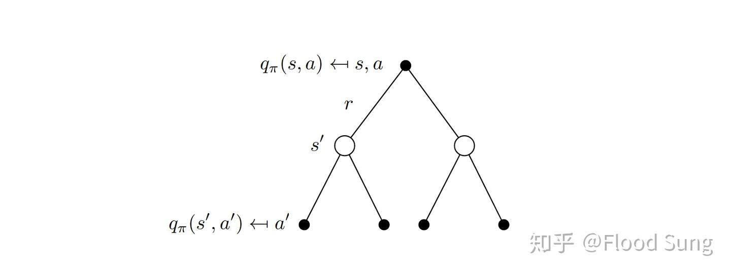
Figure: Bellman Equation

我们常见的对于Q函数的Bellman equation是这样的：

\[q_{\pi}(s, a) = r(s, a) + \gamma \sum_{s'} p(s'|s, a) v_{\pi}(s') \tag{4.5}\]

那么对于 Stochastic policy $\pi$，我们可以将其改写为：

\[q_\pi(s, a) = r(s, a) + \gamma \sum_{s'} P^a_{ss'} \sum_{a'} \pi(a' \mid s') q_\pi(s', a')\]

where

• r(s, a) 是在状态 $s$ 下采取动作 $a$ 的奖励, reward of taking action $a$ in state $s$.
• $P^a_{ss’}$ 是在状态 $s$ 下采取动作 $a$ 转移到状态 $s’$ 的概率, probability of transition from state $s$ to state $s’$ given action $a$. $P^a_{ss’} = P(s’ \mid s, a)$
• 正是第二项 $\sum_{a’}$ 的部分，incorporates the expectation over the policy $\pi(a’ \mid s’)$.
• $q_\pi(s’, a’)$ is Soft Q-value for future state-action pairs. The recursive component of the Bellman equation — provides the basis for dynamic programming. 它是一个递归的方程，提供了动态规划的基础。

对于 Maximum entropy 的目标，SAC 的做法是将 entropy 作为 reward 的一部分，而q值函数的定义也相应地进行了修改（回忆动作价值函数Q的定义，就是在当前状态下采取动作a的期望回报，而回报是当前状态下采取动作a的奖励加上未来状态的期望回报）。

我们首先回顾一下，对于一个离散的随机策略(discrete stochastic policy) $\pi(a \mid s)$，the Shannon entropy of the policy is defined as:

\[\mathcal{H}(\pi(\cdot \mid s)) = -\sum_a \pi(a \mid s) \log \pi(a \mid s) \tag{4.6}\]

This measures the uncertainty or randomness of the policy at state $s$

• Higher entropy → more randomness (uniform policy)
• Lower entropy → more certainty (greedy policy)

Now recall a key result from probability theory:

The expectation of a function $f(a)$ under distribution $\pi(a \mid s)$ is:

\[\mathbb{E}_{a \sim \pi} [f(a)] = \sum_a \pi(a \mid s) f(a) \tag{4.7}\]

So apply this to entropy:

\[\begin{align*} \mathcal{H}(\pi(\cdot \mid s)) &= -\sum_a \pi(a \mid s) \log \pi(a \mid s) \\ &= -\mathbb{E}_{a \sim \pi} \left[ \log \pi(a \mid s) \right] \end{align*} \tag{4.8}\]

Thus, entropy can be equivalently expressed as a negative expectation over log-likelihood:

\[\mathcal{H}(\pi(\cdot|s)) = -\sum_{a} \pi(a \mid s) \log \pi(a \mid s) = -\mathbb{E}_{a \sim \pi} \left[ \log \pi(a \mid s) \right] \tag{4.9}\]

之后我们将 entropy 的计算加入原本的 q 值函数中，得到 Soft Q-value function:

\[q_{\pi}(s,a)=r(s,a) + \gamma \sum_{s'} P^a_{ss'} \sum_{a'} \pi(a'|s') \left( q_{\pi}(s',a') - \alpha \log \pi(a'|s') \right) \tag{4.10}\]

可以通过下面两张图来理解：

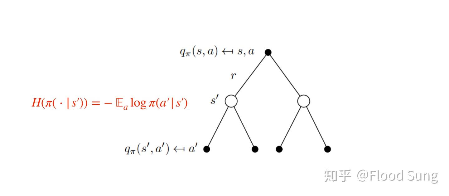
Figure: Soft Q value 1

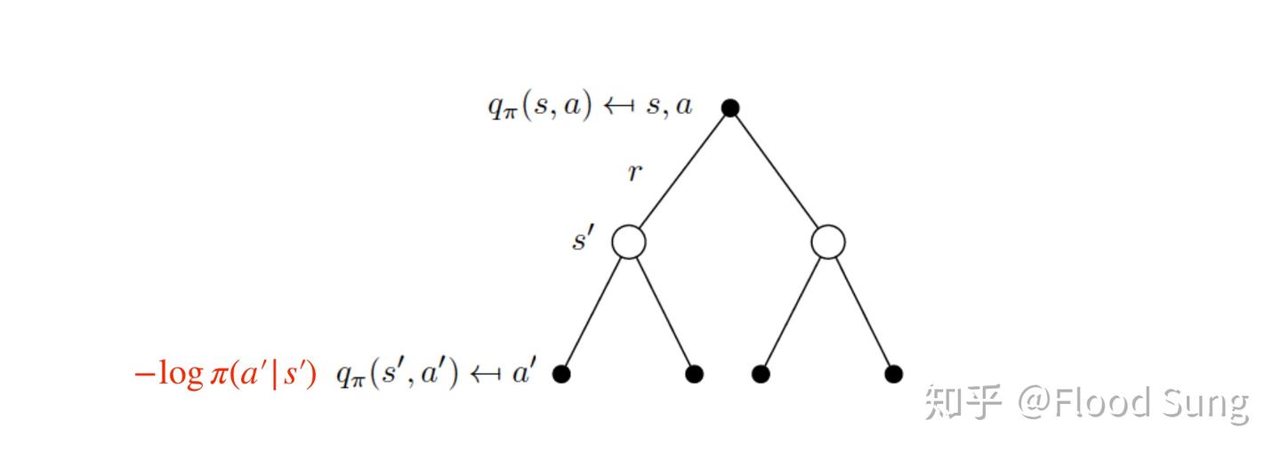
Figure: Soft Q value 2

我们知道在 Dynamic Programming Backup 中，更新 $Q$ 值的公式是：

\[Q(s, a) \leftarrow r + \gamma \mathbb{E}_{s'} \left[ Q(s', a') \right] \tag{4.11}\]

那么根据公式 4.10， 我们可以得到 Soft Bellman Backup 的公式：

\[Q_{\text{soft}}(s, a) \leftarrow r + \gamma \mathbb{E}_{s'} \left[ Q_{\text{soft}}(s', a') - \alpha \log \pi(a'|s') \right] \tag{4.12}\]

这是直接使用 dynamic programming, 将 entropy 嵌入到了 Q 值函数中计算得到的结果。

类似地，我们可以反过来把 entropy 作为 reward 的一部分，定义 Soft reward function:

\[r_{\text{soft}}(s, a) = r(s, a) - \alpha \log \pi(a|s) \tag{4.13}\]

那么我们把 式4.13 带入到 dynamic programming backup 中，同样可以得到 Soft Bellman Backup 的公式：

\[\text{derive this later}\]

同时，我们知道：

\[Q_{s,a} = r_{s,a} + \gamma \mathbb{E}_{s'} \left[ V_{s'} \right] \tag{4.14}\]

因此就有 Soft value function 的定义：

\[V_{\text{soft}}(s) = \mathbb{E}_{a \sim \pi} \left[ Q_{\text{soft}}(s, a) - \alpha \log \pi(a|s) \right] \tag{4.15}\]

至此我们理清了论文中的两个式子，即本文中的式4.3和式4.4。

好，我们回到论文中。

Lemma1 Soft Policy Evaluation

In the policy improvement step, we update the policy towards the exponential of the new soft Q function. This particular choice of update can be guaranteed to result in an improved policy in terms of its soft value. Since in practice we prefer policies that are tractable, we will additionally restrict the policy to some set of policies $\Pi$ , which can correspond, for example, to a parameterized family of distributions such as Gaussians.

我们刚刚其实已经论证过了 Soft 的部分，不过正如最前沿：深度解读Soft Actor-Critic 算法中提到的，

我们注意到上面的整个推导过程都是围绕maximum entropy，和soft 好像没有什么直接关系。所以，为什么称为soft？哪里soft了？以及为什么soft Q function能够实现maximum entropy？

理解清楚这个问题是理解明白soft q-learning及sac的关键！ SAC这篇paper直接跳过了soft Q-function的定义问题，因此，要搞清楚上面的问题，我们从Soft Q-Learning的paper来寻找答案。

参考 BAIR blog post on Soft Q-learning：

A multimodal Q-function.

这张图很明显说明了 stochastic policy 的好处，面对多模的 Q function，传统的 RL 只能收敛到一个 max 选择，而更优的办法是右图，让 policy 也直接符合 Q 的分布。

右图 (b) 中使用了指数函数的形式，

\[\pi(a \mid s) \propto \exp Q(s, a)\]

这其实来自 Boltzmann distribution，可以先将策略写为：

\[\pi(a \mid s) \propto \exp (-\epsilon (s,a))\]

其中 $\epsilon$ 是能量函数，将 $-f(x) = \epsilon$，可以有 Energy based model 的形式：

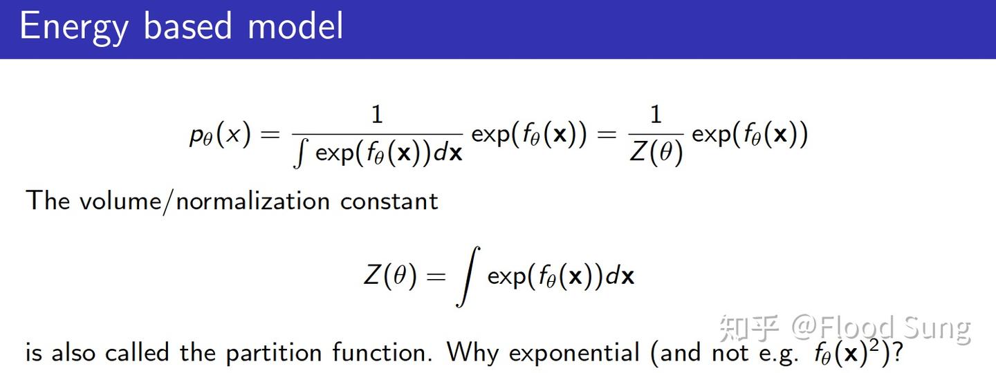
Figure: Energy based model

We start from energy-based form:

\[\pi(a \mid s) \propto \exp \left( -\mathcal{E}(s, a) \right)\]

Now, if we define the energy function as the negative of the Q-function, i.e.,

\[\mathcal{E}(s, a) = -Q(s, a)\]

Then the policy becomes:

\[\pi(a \mid s) \propto \exp(Q(s, a))\]

我们要发现该式的形式正好就是最大熵RL的optimal policy最优策略的形式，而这实现了soft q function和maximum entropy的连接。 This is the maximum entropy optimal policy form — also known as the Boltzmann (Gibbs) policy.

However, in practice, to control the stochasticity, we introduce a temperature parameter $\alpha$:

\[\pi(a \mid s) \propto \exp\left( \frac{1}{\alpha} Q(s, a) \right)\]

or

\[\pi(a \mid s) = \frac{1}{Z(s)} \exp\left( \frac{1}{\alpha} Q(s, a) \right) \tag{4.16}\]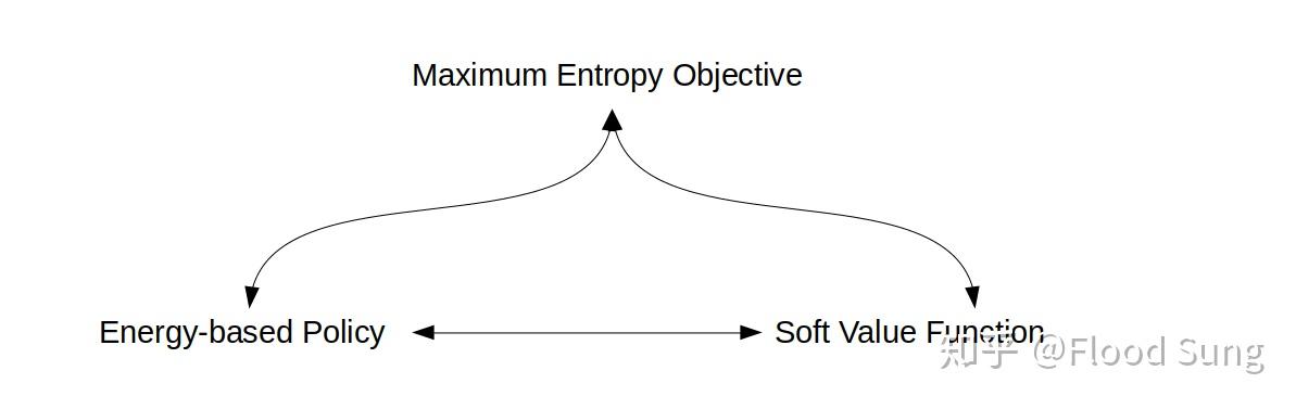

Figure: EBP, SVF and MEO

Lemma1 (Soft Policy Evaluation)

Given a policy $\pi$, the sequence of Q-functions $Q^k$ defined recursively by

\[Q^{k+1}(s, a) \leftarrow r(s, a) + \gamma \mathbb{E}_{s' \sim p} \left[ \mathbb{E}_{a' \sim \pi} \left[ Q^k(s', a') - \alpha \log \pi(a' \mid s') \right] \right]\]

converges to the soft Q-function of $\pi$:

\[Q^\pi(s, a) = \lim_{k \to \infty} Q^k(s, a)\]

所以最终，policy evaluation 用的 Soft Q function 就是我们之前定义的：

\[Q^\pi(s, a) = r(s, a) + \gamma \mathbb{E}_{s'} \left[ \mathbb{E}_{a' \sim \pi} \left[ Q^\pi(s', a') - \alpha \log \pi(a' \mid s') \right] \right] \tag{4.17}\]

展开后就是 式4.3 和式4.4。

policy evaluation 就是固定 policy，通过 Bellman backup 迭代计算得到 soft Q function 直到收敛。 下一步的 policy improvement 就是基于当前的 soft Q function 来更新策略。

Lemma2 Soft Policy Improvement

现在我们进入 Soft Policy Iteration 的第二步 —— 策略改进（policy improvement）。在这一步中，我们希望基于当前策略的软Q值 $Q^{\pi_{\text{old}}}(s, a)$ 得到一个更优的策略 $\pi_{\text{new}}$。

具体地，我们将目标策略 $\pi_{\text{new}}$ 选为最小化 KL 散度（Kullback-Leibler divergence）到 soft Q-function 指定的 Boltzmann 分布：

\[\pi_{\text{new}}(\cdot \mid s_t) = \arg\min_{\pi' \in \Pi} D_{\text{KL}} \left( \pi'(\cdot \mid s_t) \Big\| \frac{1}{Z^{\pi_{\text{old}}}(s_t)} \exp\left( \frac{1}{\alpha} Q^{\pi_{\text{old}}}(s_t, \cdot) \right) \right) \tag{4.18}\]

这就是 Soft Actor-Critic Algorithms and Applications 中的 式4。

where

• $Z^{\pi_{\text{old}}}(s_t)$ 是归一化常数，确保 $\pi_{\text{new}}$ 是一个合法的概率分布。原文中称之为 partition function that normalizes the distribution, and while it is intractable in general, it does not contribute to the gradient with respect to the new policy and can thus be ignored. 对梯度没有贡献，因此可以忽略。 \(Z^{\pi_{\text{old}}}(s_t) = \int_a \exp\left( \frac{1}{\alpha} Q^{\pi_{\text{old}}}(s_t, a) \right) da\)
• 引入了 KL divergence 来限制新策略 $\pi_{\text{new}}$ 和旧策略 $\pi_{\text{old}}$ 之间的差异，选择最小化 KL divergence 的新策略。
• $\pi’(\cdot \mid s_t)$ 是我们从策略族 $\Pi$ 中选择的候选策略，通常为一类参数化分布，例如高斯分布族。
• 右侧的 目标分布 是 soft Q 函数指定的 Boltzmann 分布，即： \(\pi^*(a \mid s) \propto \exp\left( \frac{1}{\alpha} Q^{\pi_{\text{old}}}(s, a) \right)\)

Why KL Divergence?

该投影是将目标的 Boltzmann 策略 project 到我们可实现的策略族（如高斯策略）中最接近的一项：

• 它保留了 最大熵行为 的特性；
• 保证了策略的 可表达性 和 训练可行性；
• 具有良好的梯度性质和收敛性。

Lemma 2 (Soft Policy Improvement)

Let $\pi_{\text{old}} \in \Pi$ and let $\pi_{\text{new}}$ be the optimizer of the KL projection problem in Equation (4.18). Then for all $(s_t, a_t) \in \mathcal{S} \times \mathcal{A}$ with $\mid \mathcal{A}\mid < \infty$, it holds that:

\[Q^{\pi_{\text{new}}}(s_t, a_t) \geq Q^{\pi_{\text{old}}}(s_t, a_t)\]

当我们反复进行 soft policy evaluation 与 soft policy improvement 步骤时，会产生一条策略序列：

\[\pi^{(0)} \rightarrow \pi^{(1)} \rightarrow \dots \rightarrow \pi^*\]

在 tabular setting 下，该过程可被证明将收敛到最优的 maximum entropy 策略：

Theorem 1 (Soft Policy Iteration)

Repeated application of soft policy evaluation and soft policy improvement from any $\pi \in \Pi$ converges to a policy $\pi^*$ such that:

\[Q^{\pi^*}(s, a) \geq Q^{\pi}(s, a), \quad \forall \pi \in \Pi,\ (s, a) \in \mathcal{S} \times \mathcal{A}\]

现在我们对 Soft Policy Improvement 做一个总结：

• Soft policy improvement 不再是 greedy 地选择 $\arg \max_{a} Q(s,a)$，而是以最小化 KL 散度为目标，选择一个新的策略 $\pi_{\text{new}}$
• 其本质是策略朝着 Q 值分布更集中的区域靠近，但保留了一部分的熵，使策略更为鲁棒而又具有探索性
• 在连续动作空间中，我们将此想法实现为 SAC 的 actor loss，基于reparameterization trick 直接优化

4.1.2 Soft Actor-Critic

As discussed above, large continuous domains require us to derive a practical approximation to soft policy iteration. To that end, we will use function approximators for both the soft Q-function and the policy, and instead of running evaluation and improvement to convergence, alternate between optimizing both networks with stochastic gradient descent.

这就是前文提到的 function approximation，用两个 nn 分别近似 Q-function 与 policy distribution。这对于连续控制非常必要（尽管表格型方法可以解决一些离散的问题）

作者在论文中定义的这两个网络分别是：$Q_\theta(s, a)$， $\pi_\phi(a \mid s)$，网络的参数是 $\theta$ 和 $\phi$。

Critic Loss: Soft Q-function

The soft Q-function parameters can be trained to minimize the soft Bellman residual (equation 5 in SAC 2nd paper):

\[J_Q(\theta) = \mathbb{E}_{(s_t, a_t) \sim \mathcal{D}} \left[ \frac{1}{2} \left( Q_\theta(s_t, a_t) - \left( r(s_t, a_t) + \gamma \mathbb{E}_{s_{t+1} \sim p} [V_{\bar{\theta}}(s_{t+1})] \right) \right)^2 \right] \tag{4.19}\]

where the value function is implicitly parameterized through the soft Q-function parameters, and it can be optimized with stochastic gradients

• $\bar{\theta}$ are parameters of target Q-network, updated via Polyak averaging.
• the soft value function is defined as: \(V(s_{t+1}) = \mathbb{E}_{a_{t+1} \sim \pi_\phi} \left[ Q_{\bar{\theta}}(s_{t+1}, a_{t+1}) - \alpha \log \pi_\phi(a_{t+1} \mid s_{t+1}) \right]\)

The gradient of the Q loss is (equation 6 in SAC 2nd paper):

\[\nabla_\theta J_Q(\theta) = \nabla_\theta Q_\theta(s_t, a_t) \left( Q_\theta(s_t, a_t) - \left( r + \gamma \left( Q_{\bar{\theta}}(s_{t+1}, a_{t+1}) - \alpha \log \pi_\phi(a_{t+1} \mid s_{t+1}) \right) \right) \right) \tag{4.20}\]

也就是最小化 Q-function estimate 和 soft backup target 之间的均方误差，称为 soft Bellman residual；之后用 SGD 来优化 Q-function 的参数 $\theta$。

Actor Loss: Policy Improvement via KL Minimization

Instead of directly sampling from a Boltzmann distribution, SAC parameterizes the policy $\pi_{\phi}(a \mid s)$ and minimizes the soft policy loss derived from KL divergence (equation 7 in SAC 2nd paper):

\[J_\pi(\phi) = \mathbb{E}_{s_t \sim \mathcal{D},\ a_t \sim \pi_\phi} \left[ \alpha \log \pi_\phi(a_t \mid s_t) - Q_\theta(s_t, a_t) \right] \tag{4.21}\]

This loss encourages:

• High Q-value actions (maximize $Q(s,a)$ )
• High entropy (maximize $\mathcal{H}(\pi(a \mid s))$)

Reparameterization Trick for Differentiable Sampling

To enable low-variance gradient estimates, SAC reparameterizes the stochastic policy(equation 8 in SAC 2nd paper):

\[a_t = f_\phi(\epsilon_t; s_t), \quad \epsilon_t \sim \mathcal{N}(0, I) \tag{4.22}\]

The actor loss can be rewritten using reparameterization (equation 9 in SAC 2nd paper):

\[J_\pi(\phi) = \mathbb{E}_{s_t, \epsilon_t} \left[ \alpha \log \pi_\phi(f_\phi(\epsilon_t; s_t) \mid s_t) - Q_\theta(s_t, f_\phi(\epsilon_t; s_t)) \right] \tag{4.23}\]

And the gradient becomes (equation 10 in SAC 2nd paper):

\[\nabla_\phi J_\pi(\phi) = \nabla_\phi \log \pi_\phi(a_t \mid s_t) + \left( \nabla_a \log \pi_\phi(a_t \mid s_t) - \nabla_a Q_\theta(s_t, a_t) \right) \nabla_\phi f_\phi(\epsilon_t; s_t) \tag{4.24}\]

4.2 Automating Entropy Adjustment for Maximum Entropy RL

coming soon

4.3 Network Architecture and Training

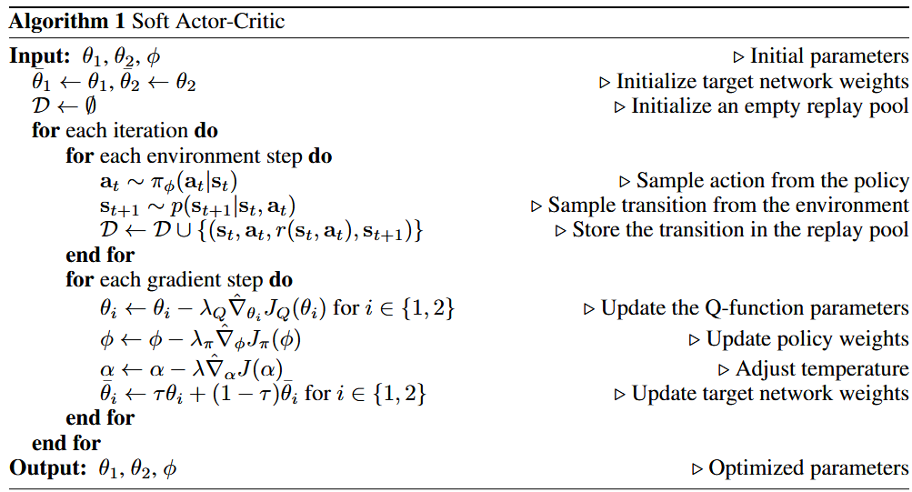
We present the Algorithm 1 table in paper Soft Actor-Critic Algorithms and Applications here:

SAC algorithm.

4.3.1 Network Architecture

SAC uses the following components:

Twin Q-Networks

To reduce overestimation bias (inspired by Double Q-learning), SAC maintains two independent Q-functions:

\[Q_{\theta_1}(s, a), \quad Q_{\theta_2}(s, a)\]

• Each outputs a scalar Q-value.
• Trained separately with identical targets.
• Only the minimum of the two is used for Actor updates and Critic targets

Stochastic Gaussian Policy Network (Actor)

The policy is modeled as a Gaussian distribution:

\[\pi_\phi(a \mid s) = \mathcal{N}(\mu_\phi(s), \sigma^2_\phi(s))\]

The network outputs mean and log std: a = tanh(μ + σ ⊙ ε), ε ∼ N(0, I), Tanh squashing ensures actions lie in bounded ranges (e.g., [−1, 1]).

Target Q Networks

For stability, SAC uses target networks for both Q-functions:

\[\bar{\theta}_i \leftarrow \tau \theta_i + (1 - \tau) \bar{\theta}_i, \quad \text{for } i = 1, 2\]

• Updated with Polyak averaging (soft target update)
• Used to compute the Bellman targets for critic loss

Temperature Parameter $\alpha$

A learnable scalar to control the trade-off between reward and entropy,

Learned via dual gradient descent:

\[J(\alpha) = \mathbb{E}_{a \sim \pi} \left[ -\alpha \log \pi(a \mid s) - \alpha \bar{\mathcal{H}} \right]\]

And automatically tunes exploration vs. exploitation.

4.3.2 Training Procedure

The SAC algorithm alternates between environment interaction and network optimization.

Collect experience from the environment:

\[a_t \sim \pi_\phi(a_t \mid s_t), \quad (s_t, a_t, r_t, s_{t+1}) \rightarrow \mathcal{D}\]

Critic update:

For each Q-function $Q_{\theta_i}$, minimize the soft Bellman error:

\[J_Q(\theta_i) = \left( Q_{\theta_i}(s, a) - \hat{y} \right)^2\]

where

\[\hat{y} = r + \gamma \left( \min_{j} Q_{\bar{\theta}_j}(s', a') - \alpha \log \pi(a' \mid s') \right)\]

Actor update:

Maximize soft Q value + entropy:

\[J_\pi(\phi) = \mathbb{E}_{s \sim \mathcal{D}, a \sim \pi_\phi} \left[ \alpha \log \pi_\phi(a \mid s) - Q_\theta(s, a) \right]\]

Temperature update:

\[J(\alpha) = \mathbb{E}_{a \sim \pi} \left[ -\alpha \log \pi(a \mid s) - \alpha \bar{\mathcal{H}} \right]\]

Target Q update:

\[\bar{\theta}_i \leftarrow \tau \theta_i + (1 - \tau) \bar{\theta}_i\]

This architecture allows SAC to be sample efficient, robust to overestimation, and suitable for high-dimensional continuous control.

Reference

• Reinforcement Learning with Deep Energy-Based Policies, Soft Q-learning
• Learning Diverse Skills via Maximum Entropy Deep Reinforcement Learning, BAIR blog post on Soft Q-learning
• Soft Actor-Critic: Off-Policy Maximum Entropy Deep Reinforcement Learning with a Stochastic Actor, the first paper of SAC
• Soft Actor-Critic Algorithms and Applications, the second paper of SAC
• 最前沿：深度解读Soft Actor-Critic 算法